Join tables
The case study
Click here, if you want to reproduce the data sets
# run these lines to create the two data sets
library(tidyverse)
set.seed(12345)
N <- 6
d <- tibble(resp_id=rep(1:N),
                name = sample(c("John", "Mary", "Mosis", "Steven"), N, TRUE),
                age = sample(30:50, N, TRUE),
                city = sample(c("Pretoria", "Cape Town"), N, TRUE),
                ans_1=sample(3,N,TRUE),
                ans_2=sample(3,N,TRUE),
                ans_3=sample(2,N,TRUE))
dt <- pivot_longer(d, cols=contains("ans"),
             names_prefix = "ans_", names_to = "question", values_to = "answer")


questions <- dt %>% select(resp_id, question, answer) %>% filter((resp_id != 4 | question!=2) & resp_id != 5)
questions <- questions %>% add_row(resp_id=7, question="1", answer=2)
demog <- dt %>% select(resp_id, name, age, city) %>% distinct()
Let’s suppose that you conducted a survey where all respondents gave some demographic informations: name, city and age.
demog
## # A tibble: 6 x 4
##   resp_id name     age city
##     <int> <chr>  <int> <chr>
## 1       1 Mary      40 Pretoria
## 2       2 Mosis     31 Cape Town
## 3       3 Steven    40 Cape Town
## 4       4 Mary      35 Pretoria
## 5       5 Steven    36 Cape Town
## 6       6 Steven    39 Cape Town
But they have answered a variable number of questions. Most have answered three questions, some have answered two, some have not answered any questions. Here is the full table of response that you captured in long format:
questions
## # A tibble: 15 x 3
##    resp_id question answer
##      <dbl> <chr>     <dbl>
##  1       1 1             1
##  2       1 2             2
##  3       1 3             2
##  4       2 1             2
##  5       2 2             3
##  6       2 3             1
##  7       3 1             3
##  8       3 2             2
##  9       3 3             2
## 10       4 1             1
## 11       4 3             2
## 12       6 1             1
## 13       6 2             1
## 14       6 3             2
## 15       7 1             2
Note also, that you have a row referring to an resp_ID =7 for which you do not have demographic information.
We will have different options to merge these two information table into one table. The package dplyr proposes a complete set of joins. As we will not use them all for our class, I am only presenting the three most common ways to join 2 tables.
If you ever need more complex ways to join tables, you are invited to consult the dplyr - joins documentation.
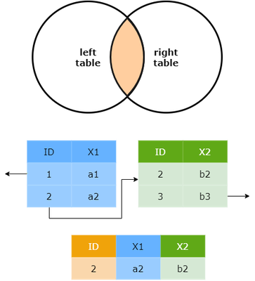
Inner join
An inner join will display all the rows from the first table that have a match in the second table.
The syntax is:
inner_join(x, y, by = ...)

# using pipe
x %>% inner_join(y, by = ...)
where x and y are two tables.
An inner join will return :
- All rows from x where there are matching values in y,
- If there are multiple matches between x and y, all combination of the matches are returned.
- All columns from x and y.
Let’s apply it to our case where the first table A corresponds to the demographics, and table B corresponds to the answers to the questions.
demog %>% inner_join(questions, by = "resp_id")
## # A tibble: 14 x 6
##    resp_id name     age city      question answer
##      <dbl> <chr>  <int> <chr>     <chr>     <dbl>
##  1       1 Mary      40 Pretoria  1             1
##  2       1 Mary      40 Pretoria  2             2
##  3       1 Mary      40 Pretoria  3             2
##  4       2 Mosis     31 Cape Town 1             2
##  5       2 Mosis     31 Cape Town 2             3
##  6       2 Mosis     31 Cape Town 3             1
##  7       3 Steven    40 Cape Town 1             3
##  8       3 Steven    40 Cape Town 2             2
##  9       3 Steven    40 Cape Town 3             2
## 10       4 Mary      35 Pretoria  1             1
## 11       4 Mary      35 Pretoria  3             2
## 12       6 Steven    39 Cape Town 1             1
## 13       6 Steven    39 Cape Town 2             1
## 14       6 Steven    39 Cape Town 3             2
As expected, the person that did not answer any of the questions will not appear in the merged table. In the same way the person ID 7 does not exist in the first table so it does not appear here, nor are the questions that are present in the table questions.
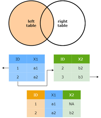
Left join
If you want the persons that did not answer questions to appear in that list, you will need to use a left join. A left_join() returns all rows from x, and all columns from x and y. Rows in x with no match in y will have NA values in the new columns. If there are multiple matches between x and y, all combinations of the matches are returned.
demog %>% left_join(questions, by = "resp_id")
## # A tibble: 15 x 6
##    resp_id name     age city      question answer
##      <dbl> <chr>  <int> <chr>     <chr>     <dbl>
##  1       1 Mary      40 Pretoria  1             1
##  2       1 Mary      40 Pretoria  2             2
##  3       1 Mary      40 Pretoria  3             2
##  4       2 Mosis     31 Cape Town 1             2
##  5       2 Mosis     31 Cape Town 2             3
##  6       2 Mosis     31 Cape Town 3             1
##  7       3 Steven    40 Cape Town 1             3
##  8       3 Steven    40 Cape Town 2             2
##  9       3 Steven    40 Cape Town 3             2
## 10       4 Mary      35 Pretoria  1             1
## 11       4 Mary      35 Pretoria  3             2
## 12       5 Steven    36 Cape Town <NA>         NA
## 13       6 Steven    39 Cape Town 1             1
## 14       6 Steven    39 Cape Town 2             1
## 15       6 Steven    39 Cape Town 3             2
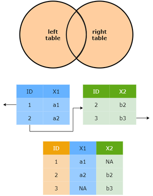
Full join
If you want the persons that did not answer questions, and the questions for which you did not have demographic information to appear, you need to apply a full_join(). As its name suggests, the full_join returns all rows and all columns from both x and y. Where there are not matching values, returns NA for the one missing.
demog %>% full_join(questions, by = "resp_id")
## # A tibble: 16 x 6
##    resp_id name     age city      question answer
##      <dbl> <chr>  <int> <chr>     <chr>     <dbl>
##  1       1 Mary      40 Pretoria  1             1
##  2       1 Mary      40 Pretoria  2             2
##  3       1 Mary      40 Pretoria  3             2
##  4       2 Mosis     31 Cape Town 1             2
##  5       2 Mosis     31 Cape Town 2             3
##  6       2 Mosis     31 Cape Town 3             1
##  7       3 Steven    40 Cape Town 1             3
##  8       3 Steven    40 Cape Town 2             2
##  9       3 Steven    40 Cape Town 3             2
## 10       4 Mary      35 Pretoria  1             1
## 11       4 Mary      35 Pretoria  3             2
## 12       5 Steven    36 Cape Town <NA>         NA
## 13       6 Steven    39 Cape Town 1             1
## 14       6 Steven    39 Cape Town 2             1
## 15       6 Steven    39 Cape Town 3             2
## 16       7 <NA>      NA <NA>      1             2
Inner, Left or Full Join ?
Most of the time, you will use the inner joins.
However, since it takes into account rows that match on both tables, it will potentially drop down some information available in one of the two tables. You have to check carefully the results obtained after a join to make sure you obtained what you wanted.
The last two types of joins will not be very useful in creating data set usable for data analysis as it potentially creates some NA cells that will introduce problems for many econometric packages.
However, the left and full joins are useful because they help you identify problems in your data sets: a NA indicates some information went missing on one of the two tables. It should trigger a question for you: is this normal ? or did I encounter some problems in the data entry (wrong ID for example). More generally, they might also be useful for specific applications.